Water Tank 6Eq
System
where
Implementation
import numpy as np
from pyrat.algorithm import ALTHOFF2013HSCC
from pyrat.dynamic_system import NonLinSys
from pyrat.geometry import Geometry, Zonotope
from pyrat.geometry.operation import cvt2
from pyrat.model import tank6eq
from pyrat.util.visualization import plot
# init dynamic system
system = NonLinSys(Model(tank6eq, [6, 1]))
# settings for the computations
options = ALTHOFF2013HSCC.Options()
options.t_end = 400
options.step = 4
options.tensor_order = 3
options.taylor_terms = 4
options.r0 = [Zonotope([2, 4, 4, 2, 10, 4], np.eye(6) * 0.2)]
options.u = Zonotope([0], [[0.005]])
options.u = Zonotope.zero(1, 1)
options.u_trans = np.zeros(1)
# settings for using geometry
Zonotope.REDUCE_METHOD = Zonotope.METHOD.REDUCE.GIRARD
Zonotope.ORDER = 50
Zonotope.INTERMEDIATE_ORDER = 50
Zonotope.ERROR_ORDER = 20
_, tp, _, _ = ALTHOFF2013HSCC.reach(system, options)
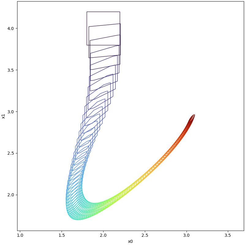
plot(tp, [0, 1])
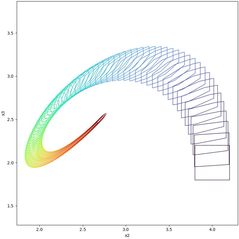
plot(tp, [2, 3])
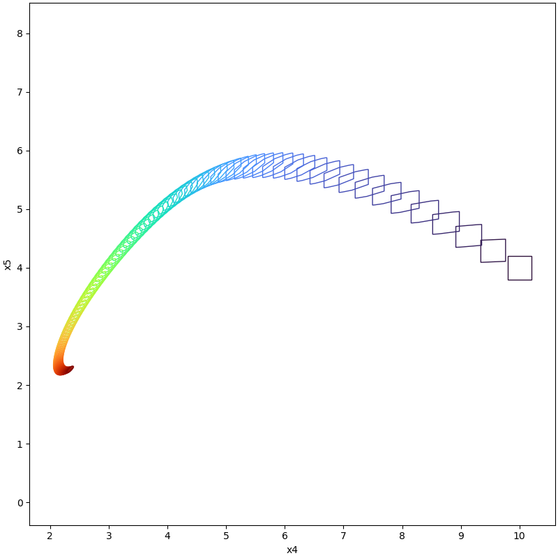
plot(tp, [4, 5])
Results