Overview

Motivation

Reachability analysis, which involves computing reachable state sets, plays a fundamental role in the temporal verification of nonlinear systems. Overly pessimistic over-approximations, however, render many temporal properties unverifiable in practice. This pessimism mainly arises due to the wrapping effect, which is the propagation and accumulation of over-approximation error through the iterative computation in the construction of reachable sets. As the extent of the wrapping effect correlates strongly with the volume of the initial set, techniques that partition the initial state space and independently compute reachable sets of those partitions are often used to reduce the wrapping effect, ${\color{red} \textrm{especially for large initial sets or/and large time horizons}}$. Such partitioning may, however, induce extensive demand on computation time and memory, often rendering the existing reachability analysis techniques not suitable for complex real-world applications. Not being forced to explore the full, i.g. exponential in the dimensionality, number of partitions could help such procedures tremendously. This is the theme of this tool, which implements the so-called 'set-boundary based method' that explores means of computing the full reachable state space based on state-exploratory analysis of just a small sub-volume of the initial state set, namely a set enclosing its boundary. For theoretical analysis, please refer to Bai Xue, Arvind Easwaran, Nam-Joon Cho and Martin Fränzle.Reach-Avoid Verification for Nonlinear Systems Based on Boundary Analysis. IEEE Transactions on Automatic Control (IEEE TAC), vol. 62: 3518--3523, 2017. and Bai Xue, Qiuye Wang, Shenghua Feng, and Naijun Zhan. Over-and underapproximating reach sets for perturbed delay differential equations. IEEE Transactions on Automatic Control (IEEE TAC), vol.66: 283--290,2020.

The set-boundary based method can be used to perform reachability analysis for systems modelled by

1. ordinary differential equations (subject to Lispchitz continuous perturbations)
2. delay differential equations (subject to Lispchitz continuous perturbations)
3. neural ordinary differential equations

Installation

The installation process is unnecessary as the source code needs to be copied into the appropriate directory, similar to how a third-party library in MATLAB works. We strongly recommend developers to utilize Pycharm as the IDE for development and testing purposes. By using Pycharm, developers can benefit from various advanced features that facilitate testing, debugging, and code analysis.

Virtual Environment

To ensure a smoother installation and running of third-party libraries, we advise users to use miniconda and create a virtual environment. The steps for this process are as follows:

First, open the user's current working directory, and use the command

conda create -n pybdr_lab

to initialize a virtual test environment called "pybdr_lab".

After the virtual environment has been created, the user needs to activate it before running any third-party libraries. This can be done using the command

conda activate pybdr_lab

By activating the virtual environment, the user ensures that any package installations and other commands will run within the virtual environment, rather than the system environment.

Dependencies

Now, the user can install the necessary third party libraries in this virtual environment using the following commands.

conda install matplotlib
conda install -c conda-forge numpy
conda install -c conda-forge cvxpy
conda install scipy
conda install -c mosek mosek
pip install pypoman
conda install -c anaconda sympy
pip install open3d

For the reason we may use Mosek as a solver for optimisation, we highly recommend you to apply for an official personal licence, the steps for which can be found at this link.

How to use

Computing Reachable Sets based on Boundary Analysis for Nonlinear Systems

The tool comes with sample files that demonstrate how it should be utilized to compute reachable sets. By referring to these sample files, users can gain an understanding of how to modify the dynamics and parameters required for reachability analysis. This feature helps users experiment with their analysis by using different settings to assess their effects on the overall computation of the reachable sets.

For example, consider the Van der Pol oscillator dynamic system:

$$\begin{align*} \dot{x} &= y \\ \dot{y} &= (1-x^2)y-x \end{align*}$$

caution

The model is already built into the model module of this tool and can be loaded directly from it. The model can be defined manually in the following way.

from sympy import *

def vanderpol(x, u):
    mu = 1

    dxdt = [None] * 2

    dxdt[0] = x[1]
    dxdt[1] = mu * (1 - x[0] ** 2) * x[1] - x[0] + u[0]

    return Matrix(dxdt)

The corresponding sample code is as follows:

import numpy as np

from pyrat.algorithm import ASB2008CDC
from pyrat.dynamic_system import NonLinSys
from pyrat.geometry import Zonotope, Interval, Geometry
from pyrat.geometry.operation import boundary
from pyrat.model import *
from pyrat.util.visualization import plot

# init dynamic system
system = NonLinSys(Model(vanderpol, [2, 1]))

# settings for the computation
options = ASB2008CDC.Options()
options.t_end = 6.74
options.step = 0.005
options.tensor_order = 3
options.taylor_terms = 4
options.u = Zonotope.zero(1, 1)
options.u_trans = np.zeros(1)

z = Zonotope([1.4, 2.4], np.diag([0.17, 0.06]))

# -----------------------------------------------------
# computing reachable sets with boundary analysis
options.r0 = boundary(z, 1, Geometry.TYPE.ZONOTOPE)
# -----------------------------------------------------
# computing reachable sets without boundary analysis
# options.r0 = [z]
# -----------------------------------------------------

# settings for the using geometry
Zonotope.REDUCE_METHOD = Zonotope.REDUCE_METHOD.GIRARD
Zonotope.ORDER = 50

# reachable sets computation
ti, tp, _, _ = ASB2008CDC.reach(system, options)

# visualize the results
plot(tp, [0, 1])

We use this setting to check the evolution of this system in the time interval [0,6.74] using a time step of 0.005, and finally, comparison between reachable sets with and without Boundary Analysis (BA) can be visualized as following:

With Boundary Analysis (BA)	No Boundary Analysis (NBA)

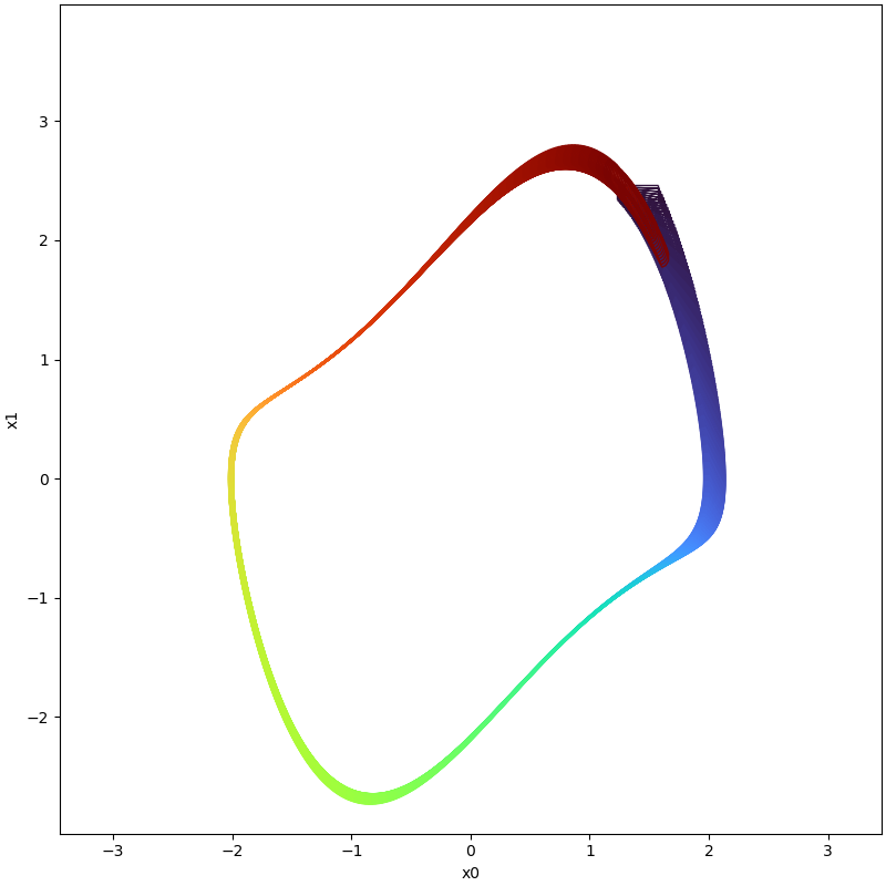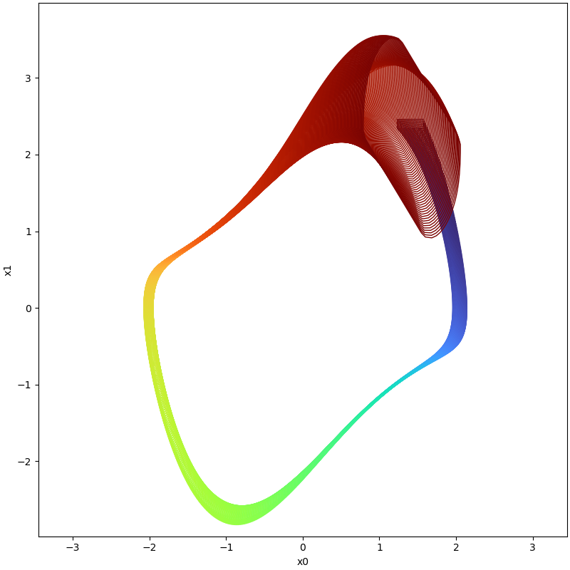For large initial sets,

System	Code	Reachable Sets (Orange-NBA,Blue-BA)
synchronous machine	benchmark_synchronous_machine_cmp.py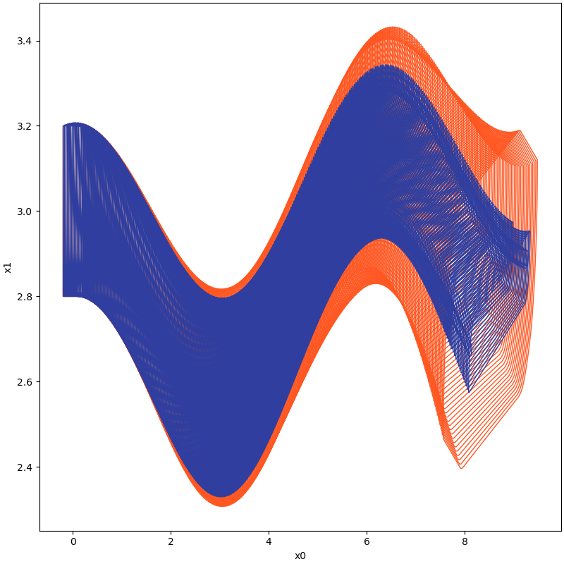
Lotka Volterra model of 2 variables	benchmark_lotka_volterra_2d_cmp.py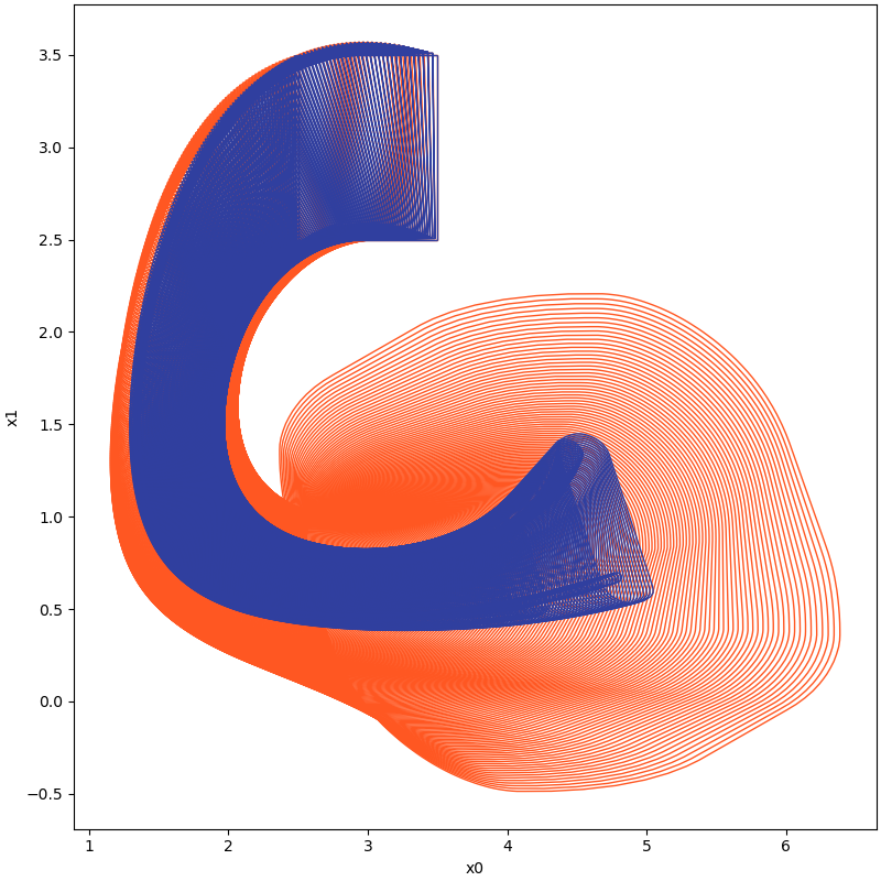
Jet engine	benchmark_jet_engine_cmp.py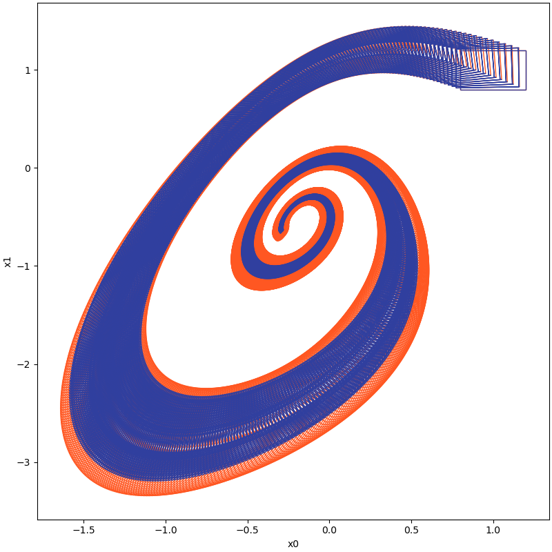

For large time horizons, i.e. consider the system Brusselator

For more details about the following example, please refer to our code.

Time instance	With Boundary Analysis	Without Boundary Analysi
t=5.4		'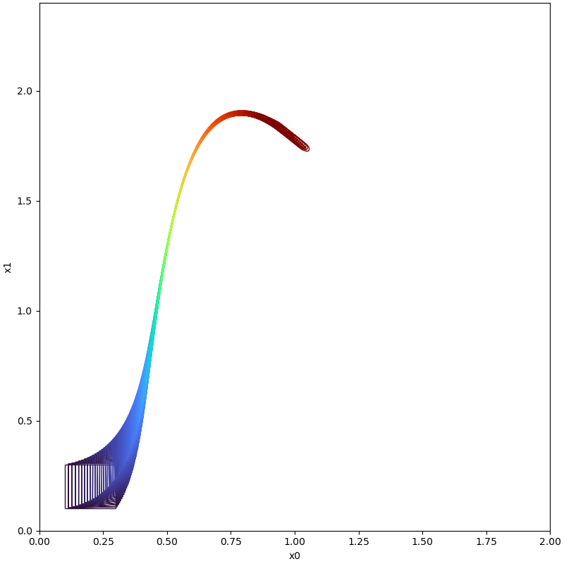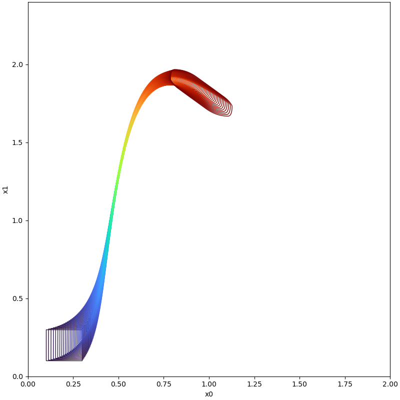
t=5.7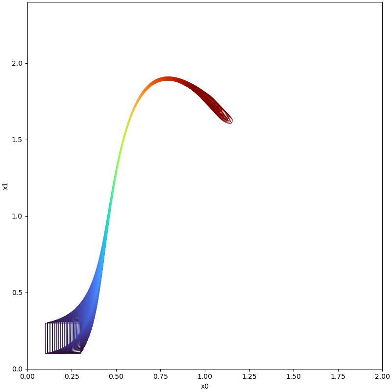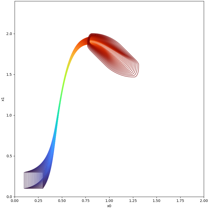
t=6.0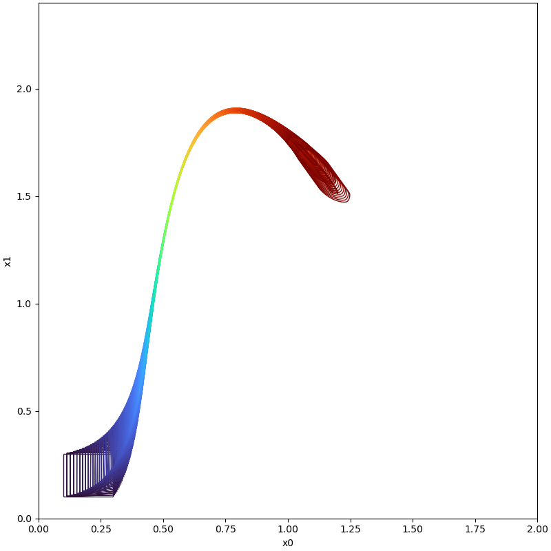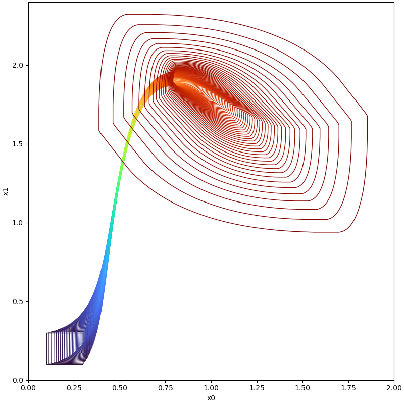
t=6.1		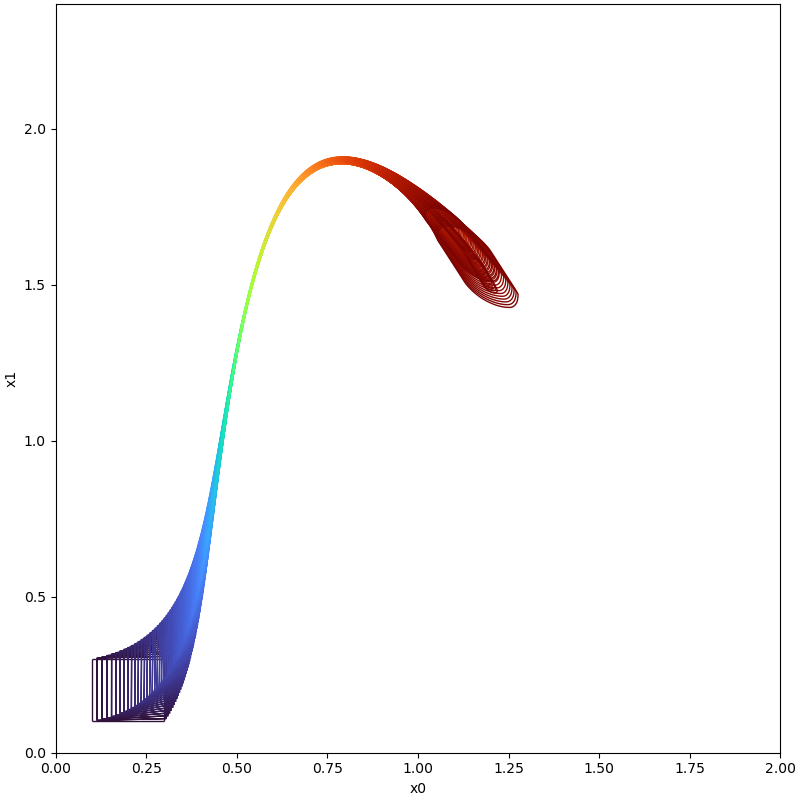Set Explosion Occurred!

Computing Reachable Sets Based on Boundary Analysis for Neural ODE

For example, consider a neural ODE with following parameters and sigmoid $\textit{sigmoid}$ activation function, also evaluated in Manzanas Lopez, D., Musau, P., Hamilton, N. P., & Johnson, T. T. Reachability analysis of a general class of neural ordinary differential equations. In Formal Modeling and Analysis of Timed Systems: 20th International Conference, FORMATS 2022, Warsaw, Poland, September 13–15, 2022, Proceedings (pp. 258-277). :

$$w_1 = \left[ \begin{align*} 0.2911133 \quad & 0.12008807\\ -0.24582624 \quad & 0.23181419\\ -0.25797904 \quad & 0.21687193\\ -0.19282854 \quad & -0.2602416 \\ 0.26780415 \quad & -0.20697702\\ 0.23462369\quad & 0.2294843 \\ -0.2583547\quad & 0.21444395\\ -0.04514714 \quad & 0.29514763\\ -0.15318371 \quad & -0.275755 \\ 0.24873598 \quad & 0.21018365 \end{align*} \right]$$

$$w_2 = \left[ \begin{align*} -0.58693904 \quad & -0.814841 & -0.8175157 \quad & 0.97060364 & 0.6908913\\ -0.92446184 \quad & -0.79249185 & -1.1507587 \quad & 1.2072723 & -0.7983982\\ 1.1564877 \quad & -0.8991244 & -1.0774536 \quad & -0.6731967 & 1.0154784\\ 0.8984464 \quad & -1.0766245 & -0.238209 \quad & -0.5233613 & 0.8886671 \end{align*} \right]$$

$$b_1 = \left[ \begin{align*} 0.0038677\quad & -0.00026365 & -0.007168970\quad & 0.02469357 & 0.01338706\\ 0.00856025\quad & -0.00888401& 0.00516089\quad & -0.00634514 & -0.01914518 \end{align*} \right]$$

$$b_2 = \left[ \begin{align*} -0.04129209 \quad & -0.01508532 \end{align*} \right]$$

import numpy as np

np.seterr(divide='ignore', invalid='ignore')
import sys

# sys.path.append("./../../") uncomment this line if you need to add path manually
from pyrat.algorithm import ASB2008CDC
from pyrat.dynamic_system import NonLinSys
from pyrat.geometry import Zonotope, Interval, Geometry
from pyrat.model import *
from pyrat.util.visualization import plot
from pyrat.util.functional.neural_ode_generate import neuralODE
from pyrat.geometry.operation import boundary

# init neural ODE
system = NonLinSys(Model(neuralODE, [2, 1]))

# settings for the computation
options = ASB2008CDC.Options()
options.t_end = 1.5
options.step = 0.01
options.tensor_order = 2
options.taylor_terms = 2
Z = Zonotope([0.5, 0], np.diag([1, 0.5]))

# Reachable sets computed with boundary analysis
# options.r0 = boundary(Z,1,Geometry.TYPE.ZONOTOPE)

# Reachable sets computed without boundary analysis
options.r0 = [Z]

options.u = Zonotope.zero(1, 1)
options.u_trans = np.zeros(1)

# settings for the using geometry
Zonotope.REDUCE_METHOD = Zonotope.REDUCE_METHOD.GIRARD
Zonotope.ORDER = 50

# reachable sets computation
ti, tp, _, _ = ASB2008CDC.reach(system, options)

# visualize the results
plot(tp, [0, 1])

In the following table, we show the reachable computed with boundary analysis and without boundary analysis on different time instance cases.

Time Instance	With Boundary Analysis	Without Boundary Analysis
t=0.5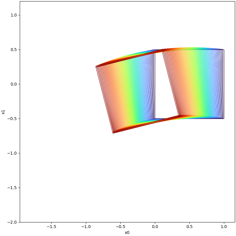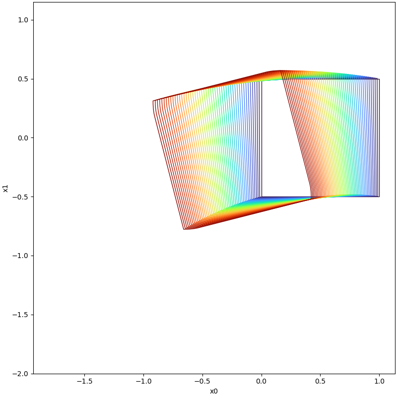
t=1.0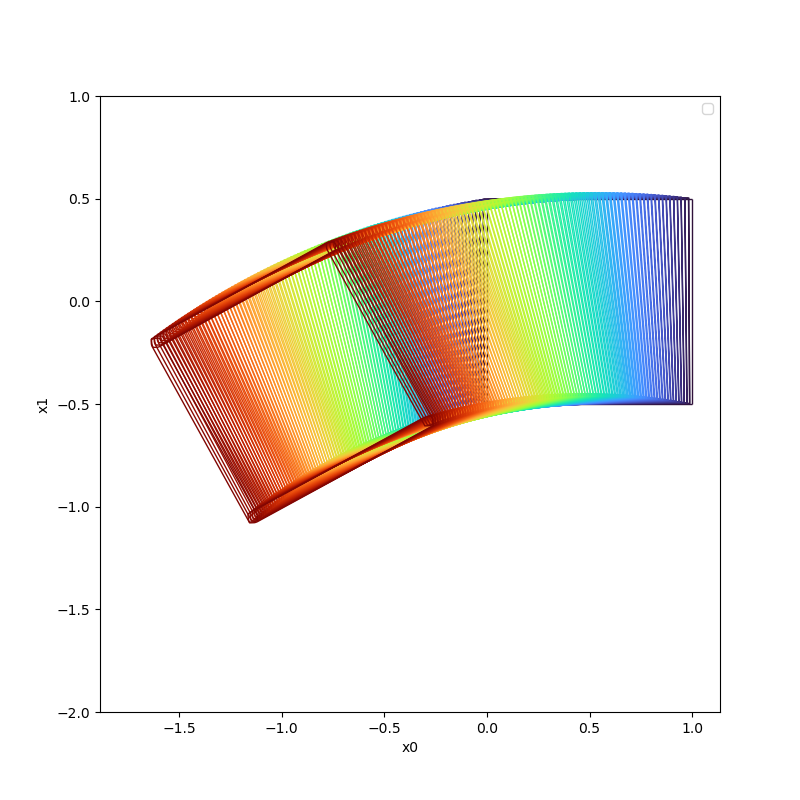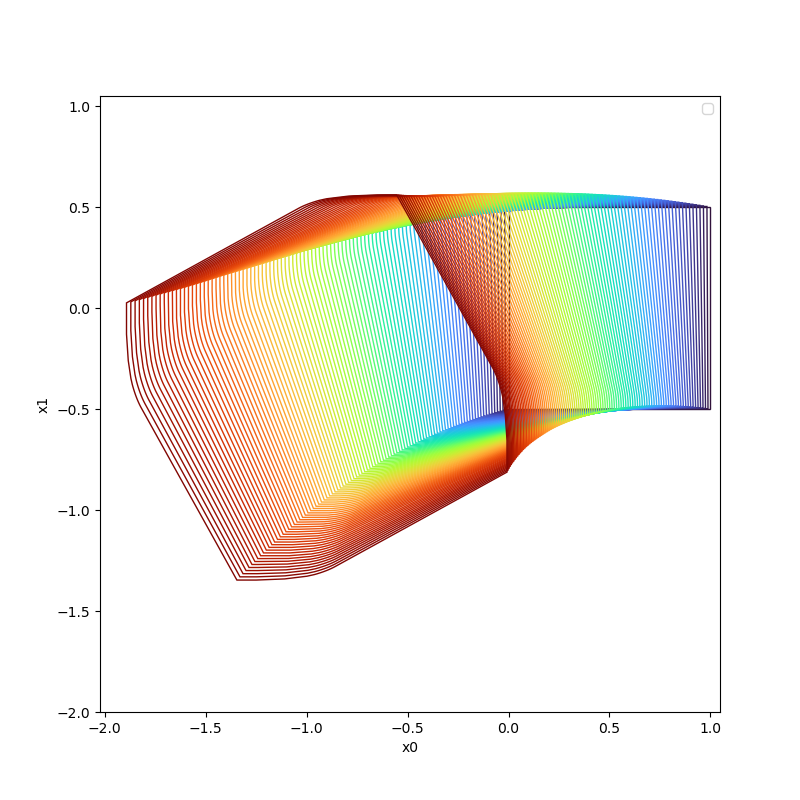
t=1.5		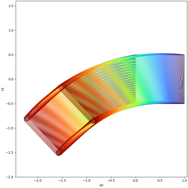Set Explosion Occured!

Misc

This tool provides necessary support to assist in the implementation of potential algorithms.

interval tensor

To enhance the calculation efficiency, this tool leverages the syntax of the third-party library numpy for interval characteristics and constructs an interval tensor to facilitate interval arithmetic. This data structure inherits numpy's syntax features and enables interval tensor computation with the broadcast mechanism, enabling parallel calculation of interval data.`

interval compatible symbolic operations

Symbolic calculation extensively utilizes the third-party library sympy. To compute the reachable set of a non-linear system via set propagation, a Taylor expansion approximation of the system at the selected state point is necessary. Therefore, this tool offers arbitrary order derivative operations of the system using sympy. Additionally, in conjunction with the interval tensor data structure mentioned earlier, the tool supports both real-valued and interval operations for the high-dimensional derivative tensor computed through symbolic calculation. Combining these capabilities simplifies the implementation of subsequent algorithms for reachable set calculation.

dynamic models

The tool has internal testing for typical dynamic models used in academic research, which can be found in the module model.

visualization

To simplify reachability analysis and enhance the presentation of computed reachable sets, we offer a basic visualisation API that has already been implemented in the visualisation module.

Frequently Asked Questions and Troubleshooting

the computation is slow

Two modes of computation are supported by the tool for reachable sets. One mode is to compute the reachable set of evolved states using the entire initial set in a set propagation manner, while the other mode is to compute the reachable set of evolved states based on the boundary of the initial state set.

The computation may be slow for several reasons such as large computational time intervals, small steps, high Taylor expansion orders, or a large number of state variables.

To accelerate the computations, experiments can be performed with a smaller computational time horizon, a smaller order of expansion (such as 2), and a larger time step. Then gradually increase the computational time horizon and order of expansion based on the results of this setting to achieve the desired set of reachable states at an acceptable time consumption.

controlling the wrapping effect

To enhance the precision of the reachable set computation, one can split the boundaries of initial sets or increase the order of the Taylor expansion while reducing the step size.

RuntimeWarning: divide by zero encountered in true_divide

This warning may appear on platforms using the Windows operating system. However, it won't impact the operation of the tool and can be eliminated by declaring it.

numpy.seterr(divide='ignore', invalid='ignore')

Feel free to contact dingjianqiang0x@gmail.com if you find any issues or bugs in this code, or you struggle to run it in any way.

Citing PyBDR

@inproceedings{ding2024pybdr,
  title={PyBDR: Set-Boundary Based Reachability Analysis Toolkit in Python},
  author={Ding, Jianqiang and Wu, Taoran and Liang, Zhen and Xue, Bai},
  booktitle={International Symposium on Formal Methods},
  pages={140--157},
  year={2024},
  organization={Springer}
}

Acknowledgement

When creating this tool, reference was made to models utilized in other reachable set calculation tools such as Flow*, CORA, and others.