Laub Loomis
System
Implementation
# init dynamic system
system = NonLinSys.Entity(LaubLoomis())
# settings for the computation
options = ASB2008CDC.Options()
options.t_end = 20
options.step = 0.04
options.tensor_order = 2
options.taylor_terms = 4
options.r0 = [Zonotope([1.2, 1.05, 1.5, 2.4, 1, 0.1, 0.45], np.eye(7) * 0.01)]
options.u = Zonotope([0], [[0.005]])
options.u = Zonotope.zero(1, 1)
options.u_trans = np.zeros(1)
# settings for using geometry
Zonotope.REDUCE_METHOD = Zonotope.METHOD.REDUCE.GIRARD
Zonotope.ORDER = 50
tps = ASB2008CDC.reach(system, options)
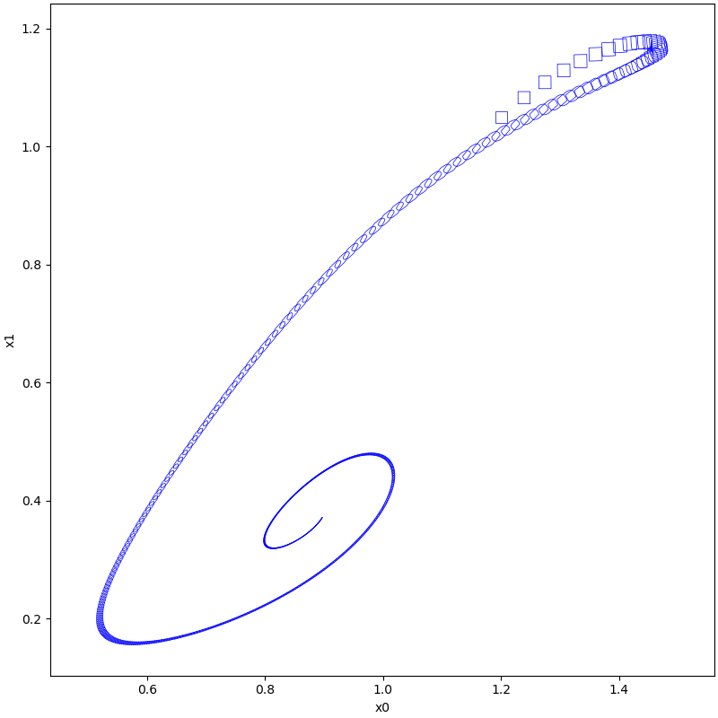
plot(tps, [0, 1])
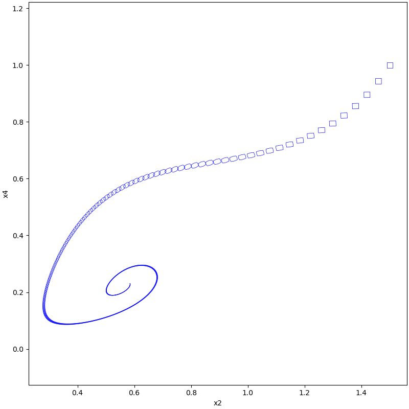
plot(tps, [2, 4])
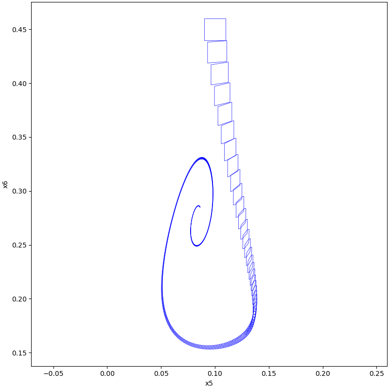
plot(tps, [5, 6])
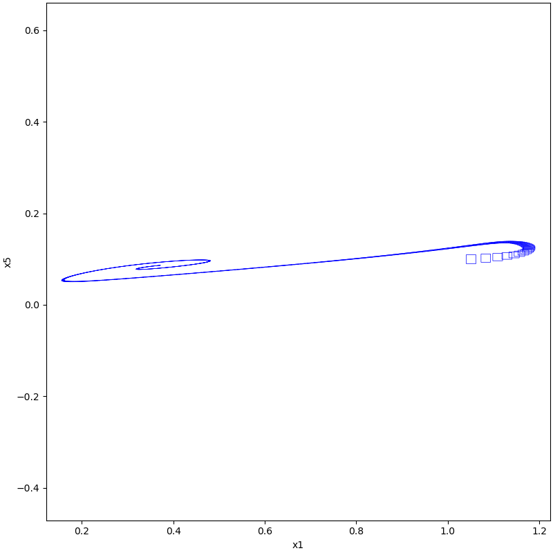
plot(tps, [1, 5])
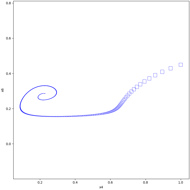
plot(tps, [4, 6])
Results